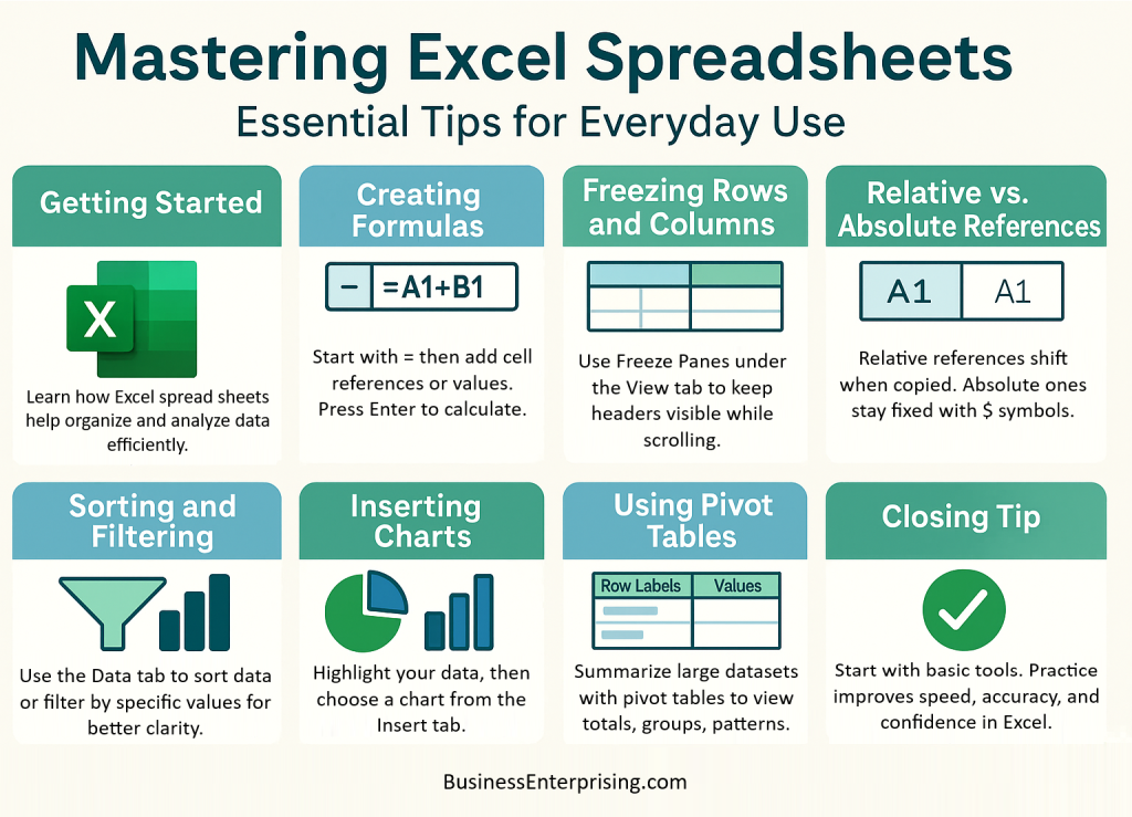
Learning how to work with Excel spread sheets can help you handle data more efficiently. The tools are simple once you know them. You can create formulas, sort lists, or build charts without much effort. These features are useful across many tasks.

Therefore, getting familiar with Excel can save you time at work. You’ll be able to organize and review information more clearly. Additionally, you can update data quickly without having to redo your work. Small changes often lead to better accuracy.

However, Excel can feel overwhelming when you first open it. The rows, columns, and buttons seem confusing until you try them. Once you begin, though, it becomes easier. You’ll start to understand how each tool helps you manage tasks.

Moreover, starting with the basics helps you build confidence. Begin by learning formulas, filters, and freeze panes. These features make a big difference in everyday use. As a result, you’ll spend less time guessing and more time getting results.

You don’t need advanced training to benefit from Excel. Focus on using the tools that match your current needs. Over time, your skills will grow as you practice. Additionally, you can learn new functions as your projects expand. Therefore, taking time to learn Excel step by step is worth it. Each new skill makes your work faster and easier. And with a little practice, you can do more than you might expect.

How do I create a formula in Excel?

Type an equals sign (=), followed by the desired mathematical expression or function, then press Enter.

Creating a formula in Excel is easier than it might seem at first. You begin by clicking the cell where you want the result. Then, type an equals sign. This tells Excel that you’re entering a formula. After that, you enter the numbers, cell references, or functions you need. For example, you can type =A1+B1 to add two numbers from those cells.

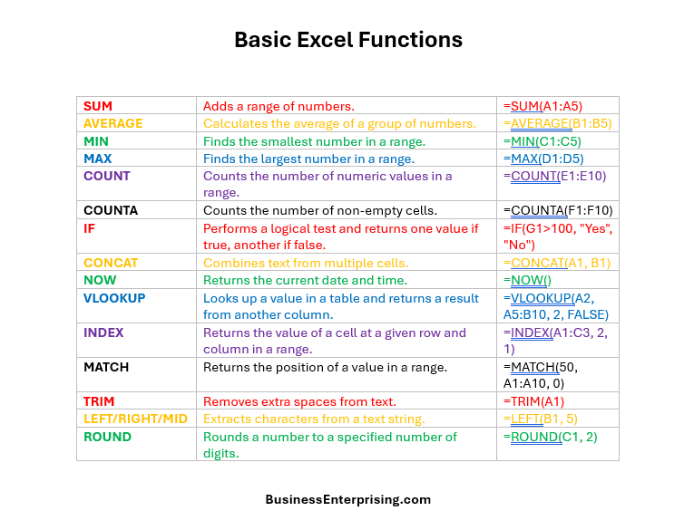
Formulas can also include built-in functions. For instance, use =SUM(A1:A5) to add all the numbers in that range. These functions save you time and reduce errors. Additionally, they can handle more complex calculations. You don’t need to memorize them all. Excel will suggest functions as you type, making the process easier.

Therefore, using formulas can improve how you work with Excel spread sheets. They help you calculate values automatically. As a result, your reports become more accurate and consistent. You can also copy formulas to other cells. This lets you apply the same calculation across many rows or columns quickly.

Moreover, it’s helpful to understand how Excel handles cell references. If you move or copy a formula, Excel adjusts the references for you. However, if you want a fixed reference, use dollar signs like $A$1. This keeps the formula pointing to the same cell.

By starting with simple formulas, you gain confidence. Then, you can explore more advanced features. But first, focus on the basics. Once you know how to enter a formula, you can do more with your data. Excel becomes a useful tool, not just a grid of numbers.

How can I freeze rows or columns?

Go to the “View” tab and click “Freeze Panes” to lock specific rows or columns in place while scrolling.

When you work with large Excel files, freezing rows or columns helps keep key information visible. This feature can save time. It also prevents you from losing track of headings as you scroll through long sheets of data.

To freeze a row or column, click the View tab on the Excel toolbar. Then, select Freeze Panes. You can choose to freeze the top row, the first column, or both. Additionally, you can freeze any specific row or column by selecting a cell and using the same menu.

Therefore, you gain more control over how your data is viewed. As you scroll, the frozen section stays in place. This makes it easier to read and compare entries across rows or columns. Moreover, frozen panes make your spreadsheets look more organized during presentations or reports.

If you want to remove the freeze, go back to the View tab. Then click Unfreeze Panes. It’s a simple way to reset your sheet layout. However, always double-check which row or column you’ve selected before freezing. It affects how your sheet will behave while scrolling.

Freezing panes is a small step, but it can make a big difference. Excel spread sheets with frozen rows or columns are easier to manage. Especially when your data gets more complex. Therefore, using this feature improves clarity and makes your work more efficient.

What is the difference between relative and absolute cell references?

Relative references change when copied, while absolute references (with $) stay fixed on the same cell.

When working with formulas in Excel, it’s important to understand how cell references behave. There are two main types to know. Relative references adjust automatically when you copy the formula to another cell. Absolute references, on the other hand, stay fixed.

Relative references are helpful when you want a formula to adapt. For example, adding values in a column becomes easier with relative references. However, sometimes you need a reference that does not change. In that case, use an absolute reference with dollar signs like $A$1.

Therefore, knowing when to use each type matters. If your formula always needs to point to the same cell, use an absolute reference. Additionally, mixed references are also possible. You can lock just the row or just the column, depending on what you need.

Moreover, using the right reference type can save you time. You avoid mistakes and reduce the need to rework your formulas. As your Excel spread sheets grow, this becomes more important. You’ll want to keep your data accurate and consistent.

To switch between reference types, you can press F4 after clicking a cell in a formula. This toggles through the options. However, always check the result to make sure it behaves as expected. It’s easy to overlook a small change when copying formulas.

Once you get used to it, the process feels natural. You’ll be able to create better formulas with fewer errors. And your work will become more efficient with every project.

How do I sort or filter data in a spreadsheet?

Use the “Sort & Filter” options in the “Data” tab to organize or limit visible data.

Sorting and filtering data in Excel helps make large sets of information easier to read. You can quickly organize data in different ways. Go to the Data tab and look for the Sort & Filter options. These tools allow you to control how your data is displayed.

Sorting changes the order of your data based on your selected column. You can sort from A to Z or largest to smallest. Additionally, you can apply custom sorts for more specific needs. However, always double-check that your headers are included to avoid sorting errors.

Filtering helps you narrow down what you see. You can display only the rows that meet certain criteria. Therefore, filtering makes it easier to focus on relevant data. For example, you might show only rows with a specific date or category.

Moreover, sorting and filtering do not change the actual data. They simply affect how the data appears in your sheet. This makes it easier to find information and review patterns. As a result, your Excel spread sheets become more functional and efficient.

To clear a filter or sort, go back to the Data tab. Then choose Clear to return your sheet to its full view. However, remember that filtered-out rows are still there. You just don’t see them until the filter is removed.

Once you get comfortable with these tools, you’ll work faster. Your data becomes easier to understand. And your spreadsheets stay organized no matter how much information you add.

How can I create a chart or graph from my data?

Select your data, go to the “Insert” tab, and choose a chart type to visually represent your information.

Creating a chart or graph in Excel helps you understand your data faster. Charts offer a clear visual of patterns and trends. First, select the cells that include the data you want to display. Then, go to the Insert tab on the toolbar.

From there, choose the chart type that fits your needs. You can pick a bar, line, pie, or column chart. Additionally, Excel gives you quick preview options to help you decide. However, try to keep your chart simple so it stays easy to read.

Therefore, it’s helpful to label your chart clearly. Add titles and axis labels to make the chart more informative. You can also adjust colors, fonts, and styles. These edits make your chart match the rest of your Excel spread sheets.

Moreover, charts update automatically when your data changes. This feature keeps everything consistent without extra effort. As a result, your reports stay current and accurate. You save time and avoid manual updates with every revision.

To move or resize a chart, click and drag it on the sheet. You can also copy it into presentations or emails. However, make sure it fits the context where you use it. You want the information to remain clear to others.

With just a few steps, you can turn raw numbers into visuals. This helps you explain your data better. And your spreadsheets become more useful for both you and your team.

What is a pivot table and how do I use it?

A pivot table summarizes large datasets, allowing you to quickly analyze, group, and filter information dynamically.

A pivot table is a powerful tool that helps you analyze large amounts of data quickly. It organizes details into a readable format. You start by selecting your dataset, then choose PivotTable from the Insert tab in the toolbar.

From there, you decide how to arrange the data. Drag fields into rows, columns, values, or filters as needed. Therefore, you can group, sort, and total the data without writing any formulas. Additionally, you can adjust the layout to show trends or comparisons.

However, keep your original table well-structured. Clean data helps the pivot table work more effectively. You should label each column clearly before creating it. This makes it easier to select the right fields during setup.

Moreover, pivot tables update as your data changes. You can refresh them with one click to reflect the latest inputs. As a result, they help you maintain accuracy while saving time. Excel spread sheets become more dynamic and flexible when you use this feature.

You can also filter pivot tables to narrow your results. For example, you might look at sales by region or totals by month. Additionally, formatting options allow you to highlight values or adjust styles. These edits help your reports stand out.

Once you get used to pivot tables, you’ll use them often. They reduce manual sorting and give you clear answers faster. Your spreadsheets will work harder for you with minimal effort.

Conclusion

Mastering basic Excel features gives you more control over your data. You don’t need to know everything to get results. Start with small tasks like writing formulas, sorting information, or freezing headers. These steps help you build confidence with Excel spread sheets.

Therefore, learning to filter and group data improves how you work. You can organize large lists and find details faster. Additionally, using charts makes your reports more readable. Visuals often help people understand numbers at a glance.

However, some tools may take practice. Pivot tables, for example, can feel unfamiliar at first. But once you use them, they save time. You can summarize complex data with just a few clicks. Therefore, these features reduce manual work and help avoid errors.

Moreover, Excel works well for both simple and detailed tasks. It can support quick calculations or large-scale reporting. Your spreadsheets can grow with your projects. Additionally, you can revisit and update them as your needs change.

Focus on using what helps you most right now. Over time, you’ll get more comfortable. You’ll also discover which features save you time and effort. As a result, your skills will improve naturally without added pressure.

Keep exploring when you’re ready. But for now, applying what you’ve learned can already make a difference. Small improvements in how you use Excel lead to better results. And your everyday tasks can feel more manageable with just a few adjustments.